All posts by Cassie Ettinger

Recently I’ve needed to visualize spatial changes in my microbiome data that are easily interpretable by other people. The best solution I’ve come across is simply projecting the data onto a drawing of my organism. Like this:

Alpha diversity of samples from pieces of a seagrass plant projected onto a drawing of that plant.

I’ve used SitePainter to produce these in the past, and in some ways it’s great. I got the figure I wanted and I’ve received a lot of positive feedback about it. The only problem is it has a steep learning curve and is the most dysfunctional GUI I’ve ever come across (generating the figure above took several days of my time, the first time). So when it became necessary to produce over forty more images like it I decided to search for a better way.

My first instinct was that there should be an easy way…

View original post 694 more words

ASM Highlights

June 12, 2015UncategorizedASM2015Cassie Ettinger

The Seagrass Team (Hannah, Jenna & I) hit up ASM this year which was in New Orleans. In case you missed ASM, Jonathan took the effort to compile all the tweets together (#ASM2015) and his efforts can be found: here.

However in case you don’t want to wade though thousands of tweets I’ve included some some brief highlights:

NCBI’s Targeted Loci Blast (MOLE-BLAST)

Using MOLE-BLAST you can blast specific 16S or ITS sequences against NCBI currated databases for those marker genes. This seems like it could be really useful if you want to identify bacterial or fungal taxonomy using a marker gene approach. Also, MOLE-BLAST appears to use a tree based approach to help you find the nearest neighbor for taxonomy assignment.

Carl Zimmer’s Talk on Microbiomes and the Hyperbolome

His talk should have just been retitled to “Microbiomes – Ode to Jonathan Eisen’s Lab”
David Coil’s response to the beard poop debacle in Slate and the kittybiome both made it into his talk

The Session that kept Redefining the Tree of Life (aka Unearthing the Dark Matter of Microbial Metabolism and Diversity)

Unfortunately, I missed this session, but apparently both Brett Baker (@archaeal) and Laura Hug (@LAHug_) shook things up
Brett Baker brought Thorarchaeota to the party, a monophyletic group that looks like it branches between Lokiarchaeota and Eukaryotes
Then Laura Hug showed up with Woesearchaeota and Pacearcheoata, not sure where they fit in, but cool

Contributions to “Extreme” Microbiology by Female Scientists Session

The whole session was awesome (and extreme), but Emmie de Wit gave a heartfelt (and tear producing) talk on being a first responder to the Ebola outbreak in Liberia
Also, I now really want to go to the Bonneville Salt Flats that Betsy Kleba talked about

Honorable mentions: John Zehr (Talk on open ocean Nitrogen fixing symbionts), David Baltrus (Talk on fungal endophytes with bacterial symbionts in their hyphae), Michael Wagner (Talk on syntrophy between nitrite and ammonia oxiders and alternative substrates for nitrification), Tom Marshburn (A real life astronaut!), Tom Sharpton (A Shotgun Metagenome Annotation Pipeline (ShotMAP))

Hannah and I presented posters at the meeting, her poster (left, #1237) and my poster (right, #1236) can be seen below:

Of course, Team Seagrass wasn’t the only ones from the Eisen lab presenting at ASM. David Coil (@davidacoil), Srijak Bhatnagar (@srijakbhatnagar) and Megan Krusor (@MKrusor) also presented posters this year! See tweets with photos below.

Microbiome Game #ASM2015 pic.twitter.com/ZW60msEgym

— Sima Tokajian (@STokajian) June 2, 2015

I found @srijakbhatnagar sporting mic diversity shirt & preaching vermicompost to control agrobacterium #asm2015 pic.twitter.com/qgh1Ml6tqX

— Ben Roller (@ben_roller) June 2, 2015

Come to my poster at #ASM2015! No. 2135 pic.twitter.com/OXPMnIZBN3 — Megan Krusor (@MKrusor) June 2, 2015

Some might say that the real highlight of ASM was New Orleans itself; it was my first time there and I really enjoyed being immersed in the culture (the music!), city and food (especially the food). Below is a picture of me touching the Mississippi River (my first time!). Unfortunately, the water was too murky to search for any seagrass or seagrass relatives.

Fungal ITS Taxonomy Problem: SOLVED (for now)

February 23, 2015Edge Effects, Fungal ITS, Project UpdatesCassie Ettinger

The past couple weeks (maybe months?) I’ve been struggling with analyzing some fungal ITS data that we have for our Edge Effects side project. No one in our lab really specializes in fungal barcoding (or fungal anything) so we became sheep and followed the mainstream path. We amplified the ITS region, between the small subunit and large subunits of RNA, which was to our knowledge the “chosen one” for fungal barcoding, using ITS1F and ITS2 primers. ITS appears to serves its purpose in terms of detailed classification (family/genus taxonomic levels) but it is definitely not a perfect barcode – for one ITS reads cannot be aligned (perhaps due to too much variation between reads, insertions, deletions, length variation, etc) which makes the reads useless by themselves for phylogenetic approaches.

Before this particular dataset fell into my hands, it was in Jenna’s and when issues with the ITS dataset arose, she turned to twitter for answers (part 1 and part 2). The conclusion – due to our desire for phylogenetic analysis it is highly likely that future fungal analysis will not be done using ITS as ultimately we care more about phylogeny than taxonomy.

That is great – but we still have our ITS dataset, what do we do with it?

I essentially did what they do here in this tutorial which I of course found after figuring out what to do from scratch. I used the UNITE ITS database to cluster my forward unmerged reads into OTUs in QIIME using UCLUST. I also used UCLUST to assign taxonomy (because it was the default option). I then did some basic filtering using filter_taxa_from_otu_table.py and filter_otus_from_otu_table.py to remove singletons, mitochondria, chloroplasts and unassigned (at kingdom level) taxa. This is where things began to go wrong (if they weren’t already wrong to start with).

I summarized my biom table using biom summarize-table and I saw this:

Counts/Sample summary:
Min: 0.0
Max: 838.0
Median: 30.000
Mean: 100.512
Std. dev.: 201.292

What happened to all my sequences?? Better yet, are there even fungi on seagrass? Is what we are seeing the result of low fungal biomass????

Let the investigation begin. I decided to look at what my biom table looked like before I filtered out the unassigned reads. This is what I saw.

Min: 14.0
Max: 48889.0
Median: 2847.000
Mean: 6001.653
Std. dev.: 9287.627

Now, that looks a bit better… except that the “unassigned” reads could be anything (seagrass, jellyfish, bacteria, fungi, sponges, etc). Since we want to do a “fungal” analysis this just won’t do. So to investigate further, I downloaded NCBI’s nucleotide “nt” database. Approx ~4250 OTU’s in my dataset were classified as “Unassigned” so I pulled these out and locally blasted them against the “nt” database to get some idea of their taxonomy. What I found was that my “Unassigned” OTUs were seagrass, jellyfish, bacteria, sponges and lots and lots of uncultured fungi. Of my ~4250 OTU’s, ~3250 hit something in the “nt” database and ~700 of hit something with >70% identity over >70% of the query OTU length. So there are obviously fungi (or fungi-like sequences) in my dataset that aren’t being identified using the method for taxonomic assignment I’ve been using (UCLUST & UNITE).

On a whim while writing this blog post about the dreary nature of ITS, I took a second look at the earlier mentioned tutorial. On the surface, it looks identical to what I did with my dataset (reassuring), but I then noticed they were using a mysterious parameter file. Perhaps this parameter file was filled with rainbows, pixie dust and unicorns that could solve all my fungal problems? To investigate further, I downloaded and took a peak at this mythical parameter file. Cue dramatic music. Low and behold, they are using the “blast” method for taxonomic assignment over UCLUST. So I thought what the heck, I’ll try anything at this point to make this fungal data usable, let’s give it a go. Of course (because this is how my life seems to be going recently) using the “blast” method of taxonomic assignment worked like magic. My new biom table summary (and this is after removing OTUs with “No blast hit”) looks like this:

Min: 7.0
Max: 47199.0
Median: 2344.000
Mean: 5441.093
Std. dev.: 9146.485

According to the log file, using the “blast” method 4717 sequences were inspected and only 1796 could not be identified. This is a huge improvement from before where ~4250 were “Unassigned”. I will note here, that upon investigating the blast assigned taxonomies, I do see a lot of unidentified fungi so this solution might not work for you if you care about specific taxonomy. I still have to analyze this new biom table which since I can’t use phylogenetic approaches will be its own hurdle, but at least I have enough truly “fungal” data to analyze now. Thinking back on all of my struggles, I am so incredibly angry that one silly QIIME parameter was what was keeping me from moving forward. Even before this I was wary of what the default QIIME script options meant for my data, but moving forward I’ll be even more vigilant in my choice of programs and parameters. This entire situation is equal parts ridiculous, embarrassing, frustrating and dumb luck. Perhaps, the craziest part is that had I not decided to write a blog post about my problems with ITS, I would never have found the solution to this particular problem. I can’t be the only one to ever have had this issue – is this some well kept mycologist secret method to ITS success? My hope is that by writing this blog post, I can save others from weeks (or months) of mental anguish over poor quality ITS taxonomic classification when the answer is hidden (or not so hidden) away in a silly parameter file.

What’s that in my Seagrass?

October 24, 2014Uncategorized#APBioGradsky, Winograsky columnsCassie Ettinger

This past weekend we took Bethany Dixon (@MsBethDixon)’s class of AP Bio students out to Bodega Marine Laboratory to make winogradsky columns from seagrass sediments. For more information about what we were doing, why we did it and what the heck a winogradsky column is see Jenna’s previous posts, AP Bio Winogradskies and AP Bio Winogradskies Pt 2. As part of the experience, the students had to opportunity to wade out into a seagrass meadow to collect samples and thus the mysteries begin! Follow along on twitter with #APBioGradsky!

UNSOLVED MYSTERIES:

What is that I see in my seagrass roots? What is that is that sticky white stuff? Fungi? Underwater spiderweb?

When placed underwater this strange organism looks like a wiggly worm brain – what the heck is it?? Zombie slug?

AP Bio Winogradsky Recipes

October 23, 2014Uncategorized#APBioGradsky, Winograsky columnsCassie Ettinger

This past weekend we took Bethany Dixon’s class of AP Bio students from Western Sierra Collegiate Academy out to Bodega Marine Laboratory to make winogradsky columns from seagrass sediments. For more information about what we were doing, why we did it and what the heck a winogradsky column is see Jenna’s previous posts, AP Bio Winogradskies and AP Bio Winogradskies Pt 2. For more winogradsky goodness see: Adventures with Winogradskies, Further Adventures with Winogradskies, Even More Adventures with Winogradskies and On the Road Again: Adventures with Winogradskies. Keep up to date with these columns by following along on twitter with #APBioGradsky!

How to Make a Winogradsky: We gave the AP Bio class a standard winogradsky recipe and then five “experimental” recipes. These recipes are described below.

Standard (10x Recipe)
cellulose 1 g
sodium sulfate 1 g
ammonium chloride 0.1 g
calcium carbonate 0.1 g
potassium phosphate 0.1 g
diatomaceous earth 300g

This is the standard recipe which we are using for our “control” columns.

Potassium Nitrate (10x Recipe)
cellulose 1 g
sodium sulfate 1 g
ammonium chloride 0.1 g
calcium carbonate 0.1 g
potassium phosphate 0.1 g
diatomaceous earth 300g
potassium nitrate 0.1 g

This recipe adds potassium nitrate to the standard recipe. By adding potassium nitrate, we hope to encourage denitrification (the process by which microbes take in nitrate and produce N2). By encouraging denitrification, we hope to enrich for microbes potentially involved in the nitrogen cycle.
Ammonium Acetate (10x Recipe)
cellulose 1 g
sodium sulfate 1 g
ammonium chloride 0.1 g
calcium carbonate 0.1 g
potassium phosphate 0.1 g
diatomaceous earth 300g
ammonium acetate 0.1 g

This recipe adds ammonium acetate to the standard recipe. By adding ammonium acetate, we hope to encourage nitrification (the process by which microbes take in ammonia and produce nitrite). By encouraging nitrification, we hope to enrich for microbes potentially involved in the nitrogen cycle. Also ammonium acetate provides an additional carbon source for the microbes and should help encourage microbial growth.

Iron(III) Phosphate (dihydrate) (10x Recipe)
cellulose 1 g
sodium sulfate 1 g
Iron(III) Phosphate (dihydrate) 0.1 g
calcium carbonate 0.1 g
potassium phosphate 0.1 g
diatomaceous earth 300g

This recipe replaces ammonium chloride from the standard recipe with Iron(III) phosphate (dihydrate). Iron is a necessary co-factor for nitrogen fixation and both iron and phosphorus have been posited to co-limit nitrogen fixation in the ocean. By adding iron(III) phosphate, we hope to encourage nitrogen fixation (the process by which microbes take in N2 and produce ammonia). By encouraging nitrogen fixation, we hope to enrich for microbes potentially involved in the nitrogen cycle.

Seagrass Roots (10x Recipe)
Seagrass roots 1g
sodium sulfate 1 g
ammonium chloride 0.1 g
calcium carbonate 0.1 g
potassium phosphate 0.1 g
diatomaceous earth 300g

This recipe replaces cellulose from the standard recipe with seagrass roots. Since we are trying to culture seagrass associated microbes, we thought that it would be interesting to use seagrass roots as the carbon source for the winogradsky columns. We hope that this will result in an enrichment of microbes that from symbiotic relations with seagrass roots.

Elemental Sulfur (10x Recipe)
cellulose 1 g
sodium sulfate 1 g
ammonium chloride 0.1 g
calcium carbonate 0.1 g
potassium phosphate 0.1 g
diatomaceous earth 300g
elemental sulfur 0.1g

This recipe adds elemental sulfur to the standard recipe. By adding elemental sulfur, we hope to enrich for microbes involved in the sulfur cycle.

Collecting seagrass and sediment!

Inoculation: We had the students prepare their recipes on their first day and then inoculate them on their second day. We inoculated them with seagrass sediment and water collected from Bodega Bay by the AP Bio class. We mixed the sediment and water collected vigorously and let the sediment settle. The water was then used to inoculate the columns.

Inoculating our winogradskies!

The finished columns! #APBioGradsky

Lake Arrowhead: Posters, Comics and Doodles Galore!

October 4, 2014UncategorizedCassie Ettinger

Two weeks or so ago, Hannah and I presented posters on our respective seagrass microbiome work at the Lake Arrowhead Microbial Genomics meeting. Attending the meeting was a wonderful experience for both of us and the talks and people were just phenomenal! For a brief overview of each day and the accompanying storify see: Day 1, Day 2 and Day 3. Some of the talks and posters were uploaded to F1000.

On the left you can see me dutifully standing in front of my poster. On the right you can see Hannah explaining her poster to a fellow LAMG-er! Hannah’s poster is one of the ones uploaded to F1000 and can be found here.

My poster can be seen below – I took inspiration from comic books when coming up with the design.

Of course, taking inspiration from comic books then meant I was obligated to produce a comic version of my poster which you can see below!

And to conclude some of my favorite doodles from my Lake Arrowhead notes:

From Nancy Moran’s talk:

From Nicole Perna’s talk:

From Jenna Morgan Lang’s talk:

From Jeffrey Foster’s talk:

From Jennifer Gardy’s talk: (inspired by the “cat break”)

On the Road Again: Adventures with Winogradskies

October 1, 2014UncategorizedWinograsky columnsCassie Ettinger

On the Road Again: The Long Arduous Journey of Waiting for Our Microbes to Grow

Have you been waiting to hear about Winogradskies? Well, wait no more! We are here with your Winogradsky update! If you’ve forgotten what a Winogradsky column is and our goals for them I urge you to visit: Adventures with Winogradskies, Further Adventures with Winogradskies and Even More Adventures with Winogradskies to refresh your memory.

**Note all photographs in this post were taken approx. 2 weeks ago and thus the winogradskies herein described are reflective of that time point.

After 10 weeks:

These columns haven’t experienced much change except for a small increase in biomass towards the top of the layers. These three vials all still look relatively visually identical, which is reassuring as they were inoculated from the same water source and *should* be replicates of each other.

Microbial succession in action???? The two large columns that get full light (left and middle columns) were solid pink/black at 7 weeks, but now we are seeing some snow-white colored microbes intruding in. I wonder what these snow-white microbes are and what the earlier coal-black and pretty-in-pink microbes were doing metabolically that allowed the white microbes to now flourish in the columns. Alternatively, there could be no white microbes – perhaps the white is just the diatomaceous earth which is now visible again as the pink and black microbes recede into the past.

Overall, there is not a lot to report on the 5 mL tubes that were inoculated with water from different sampling locations. Except in the one above where we see a tiny band of purple!! This is the first 5 mL tube to show the presence of any pink and/or purple microbes!

Experimental Tubes (where we added either Potassium Nitrate or Ammonium Acetate) – After 9 weeks:

Overall, these tubes also look fairly similar to their 7 week incarnation. However, one of the Ammonium Acetate added vials has less black microbes at the bottom of the tube than it had previously (appearance of white microbes?). The Potassium Nitrate added vials appear to have a slight increase in the thickness of the layers.

Left to Right: Nothing Added, Ammonium Acetate Added, Ammonium Acetate Added (Kept in Dark) – Nothing Added, Potassium Nitrate Added, Potassium Nitrate Added (Kept in Dark)

The most noticeable difference is that the Ammonium Acetate added dark vial’s liquid portion has a green hue which it didn’t have before. Additionally the pinkish hue in the liquid in the Ammonium Acetate added light vial is much darker than it was before. The Potassium Nitrate vials are similar to their 7 week counterparts; they just have more biomass and/or bubbles.

Update over. Hopefully, you’ll hear from us again fairly soon with a new update on our lovable wino’s!

EDAMAME 2014’s Greatest Hits

September 2, 2014UncategorizedWorkshopCassie Ettinger

I recently had the wonderful opportunity to attend the Explorations in Data Analyses for Metagenomic Advances in Microbial Ecology (EDAMAME) Workshop. The workshop was held at the Kellogg Biological Station in Michigan by Ashley Shade (@ashley17061), Tracy Teal (@tracykteal) and Josh Herr (@number_three) – who are all AWESOME. I thought I’d go through and highlight what I found to be my favorite and/or most useful parts of the workshop.

Before I jump right in to the science, my favorite non-science related parts of EDAMAME included non-stop ice cream (lunch and dinner – with waffle cones!), meeting such a diverse crowd of microbe lovers, seeing Guardians of the Galaxy at the Alamo Drafthouse Cinema, enjoying some local Michigan beer at Bell’s Brewery and hearing Jack Gilbert (@gilbertjacka) play guitar and sing one night at the campfire (and yes, there were s’mores!).

Anyway, pop this bad boy in and let’s get started!

Track 1: O-T-U Child

For microbial ecology newbies, I think that EDAMAME’s introduction to alpha diversity and beta diversity lectures are a very good resource. I found the section on ordination plots especially helpful as even though I have taken introductory statistics classes such plots were never discussed! I would also point the microbial ecology newcomer to EDAMAME’s Introduction to Shell and Introduction to QIIME tutorials (Part 1, Part 2 and Part 3) as both are very well documented and every step in the tutorials is well described.

Some things to think about: Replication and Experimental Design. Something that was mentioned several times by different guest speakers (Pat Schloss (@PatSchloss) and Jim Cole, I think) was the idea of using a synthetic mock community each time you do a sequencing run to ascertain the error rate of that particular sequencing run. We also had several conversations about what replication means for microbial ecologists – if interested in what we discussed, go read: Replicate or lie.

Track 2: Bioinformatics Killed My Computer

If you have previously tried to pick OTU’s or chimera check in QIIME or mothur (if confused, please review resources discussed in Track 1) on your personal laptop or even a lab computer, you are probably familiar with long wait times, black screens and spinning wheels of death. Data sets are increasing in size at a much more rapid pace then the computational power included in standard use laptops. My Macbook Pro is five years old (which means its basically a dinosaur) and still kicking it with its 2.26 GHz Intel Core 2 Duo processor and its recently upgraded 8 GB of RAM. However, when it comes to some of my data analysis, its fan and slow response time make it sound like a small dying animal. So what is a researcher to do? Use a superior lab computer that has an i7 processor and 16 GB of RAM – YAY! But what happens when even that is not enough?

Solution Numero Uno: Use a service like Amazon Web Services where you pay to use Amazon’s computational power to run your analyses. Don’t know how to set up an Amazon instance? The lovely EDAMAME instructors have got you covered with this tutorial and also these follow-up tutorials on how to connect to your instance from a PC or a Mac/Linux machine. One thing that makes using Amazon Web Services nice is that there are community API’s you can use that have QIIME and/or mothur already installed.

Solution Numero Dos: Use your university’s computing cluster (if available). In my experience, most clusters are logged into the same way as you log into your Amazon instance – using SSH. For those unfamiliar with SSH, here is a tutorial I found using the magic of Google for Mac/Linux computers. One problem you might run into with using a cluster is that the software you want to use might not be installed – in which case, if you are lucky the computer gurus who manage your local cluster will install it and keep it up to date for you! However if you are unlucky… they might say that they won’t install it at all.

If using either of these solutions, I highly suggest looking into using either Screen or Tmux which were introduced to us at EDAMAME (I am currently using Tmux). Screen and Tmux allow you to open multiple bash windows on the machine you are SSH-ed into. This means if you run a command from inside a bash window in Screen/Tmux and then detach from Screen/Tmux and exit your SSH session, your command will continue to run on the server or cluster your were logged into. This means you no longer have to worry about the internet cutting out or leaving your personal computer on when running commands on remote server/clusters!

Track 3: I Wanna Download Some Genomes

Have you ever wanted to download a genome from NCBI or MG-RAST but not wanted to hassle with the ever changing website interfaces? Have you ever wanted to download hundreds of genomes but the thought of all that clicking has you wanting to run to your safe place? Me too! I found guest lecturer, Adina Chuang Howe (@teeniedeenie)’s tutorial on how to do these things from the shell to be one of the most useful parts of EDAMAME. The tutorial comes with the necessary scripts that you can re-purpose to download your favorite genomes – these could potentially save you hours and hours of valuable research time (and most of your sanity).

Track 4: I Got A Database

Throughout EDAMAME, we were introduced to several different marker gene databases (16S, ITS). The default database in QIIME is the greengenes database and until EDAMAME, I never realized just how many databases there were! I was especially surprised when in Jim Cole’s guest lecture he showed us a slide with a venn diagram comparing the sequences contained in the different fungal ITS databases and there was a definite visible discrepancy between what each database contained. I also found his slides comparing the taxonomic accuracy of the different fungal ITS databases as we have some seagrass fungal microbe data to analyze. I think the exposure to the different databases was helpful to my evolution as a microbial ecologist as it made me start thinking about which database I’m using for my analyses and what my biases these databases might introduce to my analysis. Some helpful questions to keep in mind when looking at different databases are laid out in this EDAMAME tutorial.

Track 5: Don’t You (Forget To Visualize Me)

Humans are very visually oriented creatures and having visually appealing, statistically accurate and reproducible graphs can really help a presentation succeed. A strong knowledge of R (which I someday hope to have) can help you achieve such graphs. We walked through several different R tutorials relating to microbial ecology at EDAMAME which I thought were helpful when combined with EDAMAME’s beta diversity and hypothesis testing lectures. These R tutorials were also specifically aimed at utilizing OTU tables which helped me think about how I might apply what I was learning to my own data analysis. We were also introduced to a vast array of data visualization and exploration tools (see this lecture).

Bonus Track: Hooked on Microbial Ecology (because if I hadn’t been hooked on microbial ecology before EDAMAME, I sure as would be now!)

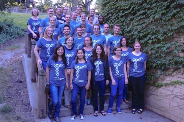
EDAMAME Class of 2014 in our MoBio T-shirts!

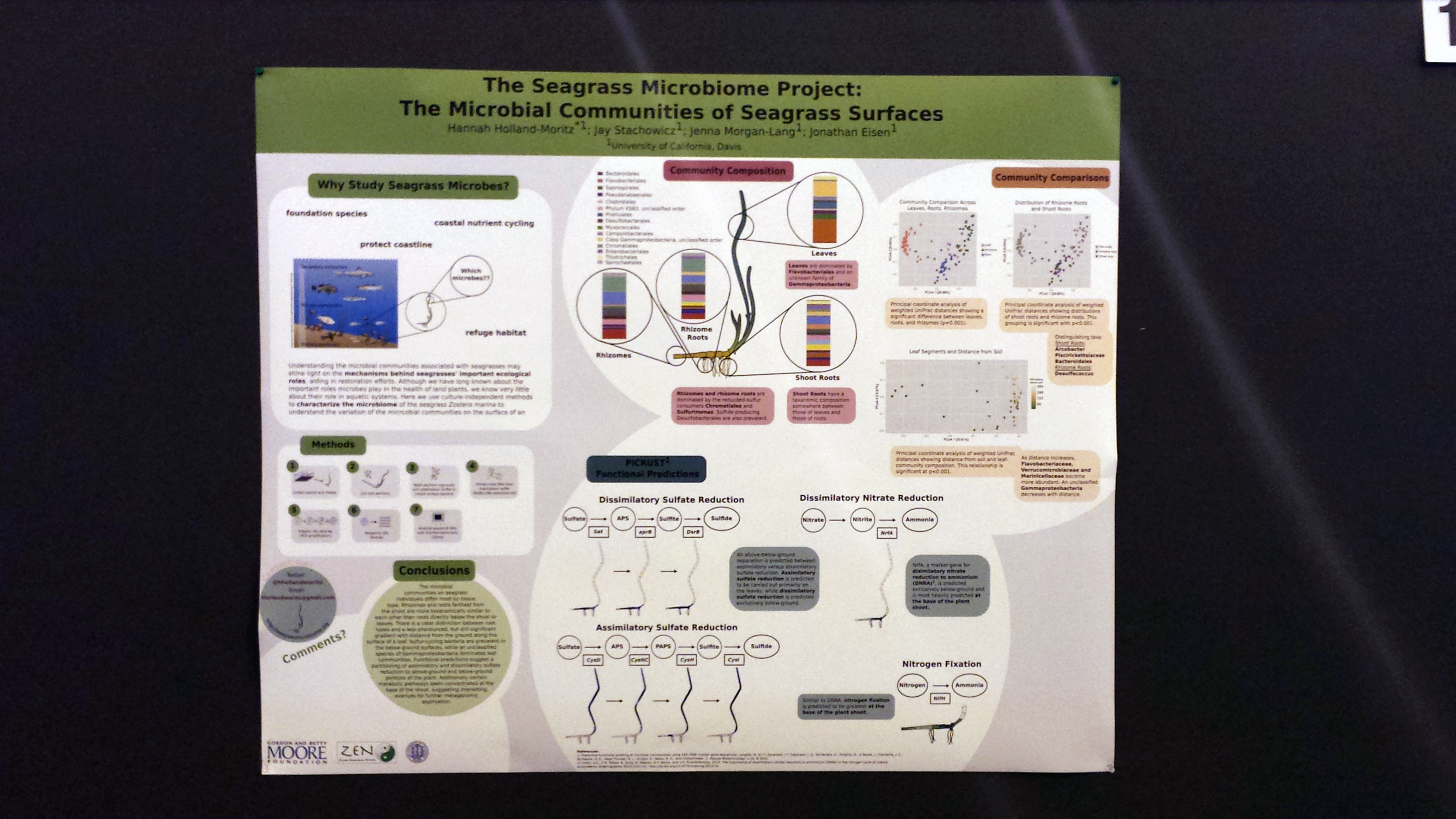
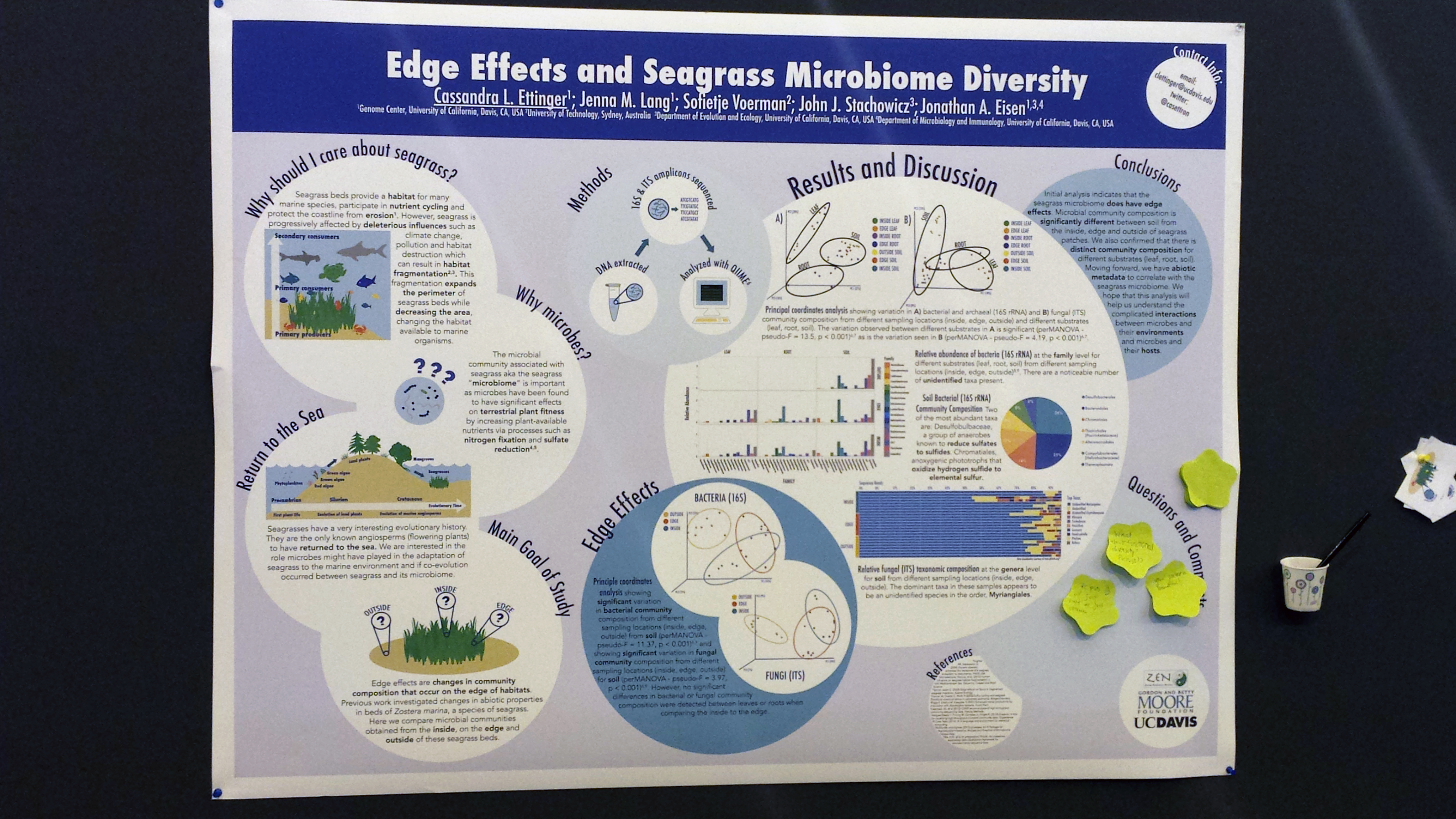
All of the workshop materials for EDAMAME 2014 can be found on their website and there is also a storify of all the live tweeting that went on throughout the EDAMAME workshop using the hashtag #edamame2014. Also, look out for a future guest post on MoBio’s blog, The Culture Dish, about seagrass microbes!

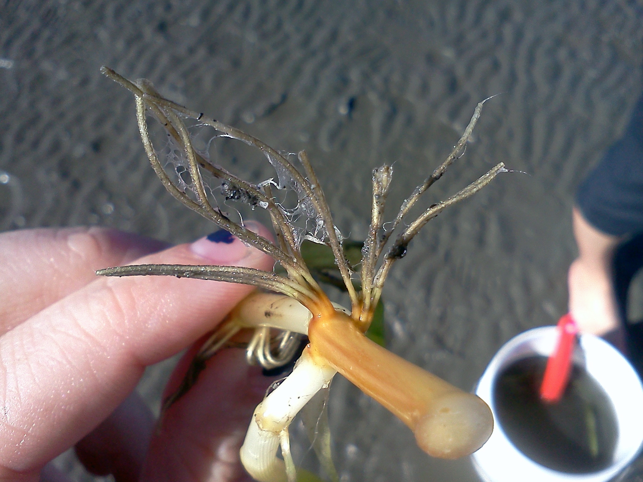
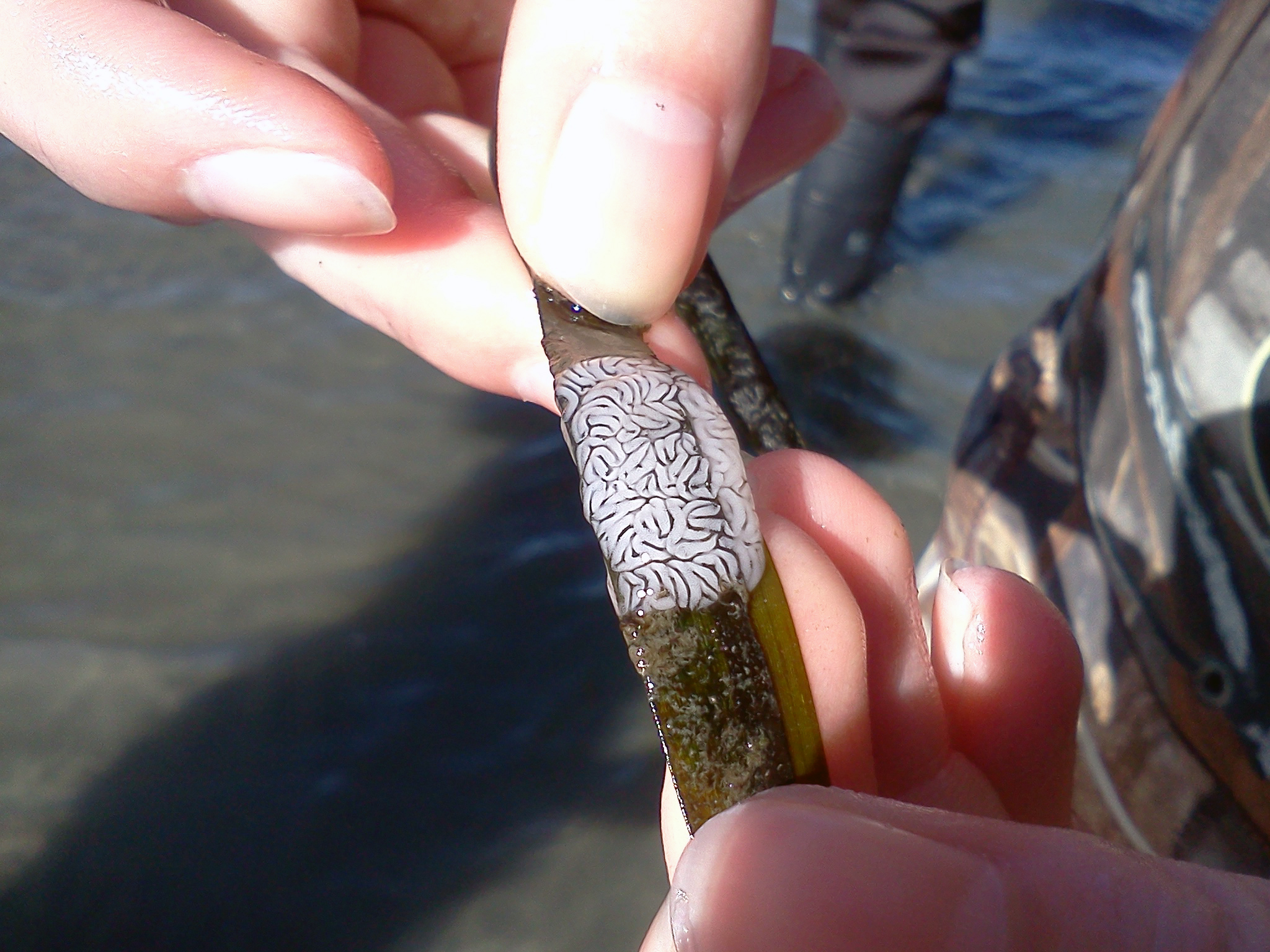
Even More Adventures with Winogradskies

August 22, 2014UncategorizedWinograsky columnsCassie Ettinger

It is time again for a Winogradsky column update! It has been three weeks since we last shared with you our Winograsky column progress. If in that time you’ve forgotten what a Winogradsky column is and our goals for them I urge you to visit: Adventures with Winogradskies and Further Adventures with Winogradskies to refresh your memory.

After 7 weeks:

We are finally starting to see some pretty pink layers! Many of the darker colored bacteria from week 4 are gone from these columns… could it be that our columns are undergoing microbial succession?? Could Winograsky columns be a good model system for studying microbial succession?

Strangely (or not so strangely?), it is our large containers that show the most variation between replicates from the same sample location. We have everything from green-as-grass and pretty-in-pink to black-as-coal microbes. The container above on the far right is the one that we’ve been simulating soil conditions in by covering the bottom half of the container – could the lack of pink and purple microbes be due to this?

Above you can see the variation in vials taken from different sampling locations. The microbes in these vials seem to be growing at a slower pace than those in the large container – we also see this with our small micro-centrifuge tubes (not pictured) which haven’t changed significantly form week 4.

Experimental Tubes ( (where we added either Potassium Nitrate or Ammonium Acetate) – After 6 weeks:

On the left are the tubes we added Potassium Nitrate too and on the right are the tubes we added Ammonium Acetate too. The Potassium Nitrate tubes have green microbes growing in firework like patterns up the sides of the tubes! The Ammonium Acetate tubes have pinkish-brown microbes clouding them up! It is amazing how different the Potassium Nitrate and Ammonium Acetate tubes are given that they came from the same original sample!

The two above tubes were kept in the dark via aluminum foil. The left tube has had Potassium Nitrate added to it and the right tube has had Ammonium Acetate added. It is hard to see but the Potassium Nitrate tube has a lot of gas bubbles in the diatomaceous earth in the bottom of the column.

Left to Right: Ammonium Acetate Added (Kept in Dark), Ammonium Acetate Added, Nothing Added – Potassium Nitrate Added (Kept in Dark), Potassium Nitrate Added, Nothing Added

The differences between the different treatments (light with chemical vs. dark with chemical vs. no chemical ) is most significant when you observe the tubes right next to each other. It will be interesting to investigate the community composition differences between all these tubes! I wonder what types of communities we’d see with different pH’s, salt concentrations or other added chemicals… Until next time, stay tuned!

Congratulations Henna!

August 14, 2014UncategorizedHigh School, Project Merccuri, Swabs to Genomes, Young Scholars Program, YSPCassie Ettinger

It has been the privilege for the Eisen lab to host Henna Hundal, a high school senior, radio show host and soon-to-be certified yoga instructor, on a six-week summer research project. Henna was part of UC Davis’ prestigious Young Scholars Program.

IMG_20140715_151631 IMG_20140630_125443

For the wet lab portion of Henna’s project, she focused on the Seagrass Microbiome which involved growing and isolating microbes from seawater on LB that she helped collect from tanks of Zostera marina at Bodega Bay.

As part of the Young Scholar’s Program, Henna had to make a scientific poster of her intended project, write a 10-30 page final paper and give a 10 minute presentation on her project. For extra credit (because Henna was magnificently studious) she also turned her powerpoint presentation into a makeshift poster.

The best explanation of Henna’s summer project was the one that Henna gave herself. As an experienced radio show host, Henna was a natural presenter. Henna’s final presentation was recorded and can be viewed: HERE.

As a whole, we are unbelievably proud of the work that Henna did while in the lab and would be happy to have her back anytime! She is an amazing young scientist and effective science communicator and we have no doubt about her future success! So congratulations Henna on being made of awesome!

The Seagrass Microbiome Project